5.3. Computing environments#
There are 2 main ways in which you can write, and execute, Python code. The first involves using a REPL [1], which I illustrate in the REPL video. This environment is most useful for experimenting with small pieces of code and, in the case of Jupyter notebooks, for interactive analyses.
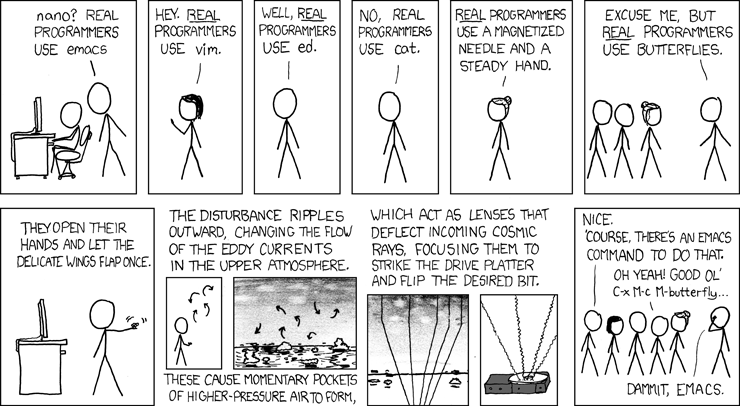
The second approach is based on writing Python scripts. A script is just a plain text file. These can be written using any program capable of saving as plain text. However, you’re strongly advised to use a “programmers editor”. There’s a multitude of these, and it’s a topic about which programmers are sufficiently opinionated as to create cartoons…

But seriously, I strongly recommend using an IDE [2] as these incorporate tools to facilitate debugging, a very useful capability (you can see a demo of this in Fixing errors). (See Setting up your own computer for installing one on your computer.)
Writing scripts has two steps for running the program (illustrated in the executing python from a text file video): (1) write the script, (2) running the script in a terminal.
5.4. Code and output in these notes is from Jupyter#
The blocks of computer code, and associated output, displayed in these notes are derived from running the code in a Jupyter notebook. Running the same code in the standard python interpreter inside a terminal will generate different looking output. The difference is most obvious on what is called the representation (or repr()) of an object. In Jupyter, the output can be “styled” (e.g. bold font, coloured tables) whereas in a conventional interpreter the output will appear as plain text (see Demonstration of using Jupyter).
5.5. Everyones first program in Python#
print("Hello World!")
Hello World!
Now that we’ve got that out of the way, let’s first treat Python as just a calculator.
5.6. Basic arithmetic operations#
5.6.1. Addition#
1 + 9
10
5.6.2. Subtraction#
1 - 9
-8
5.6.3. Multiplication#
2 * 20
40
5.6.4. Division (including integer division)#
Standard division uses a single /
20 / 3
6.666666666666667
Integer division uses //
20 // 3
6
5.6.5. Division remainder#
While integer division (a // b) returns how many times b goes into a, the modulo operation returns the remainder. This is denoted by the % symbol in Python (and many other languages). In the example, 3 goes into 20 6 times, with 2 remainder. The modulo operation only returns the latter.
20 % 3
2
The builtin divmod() returns both parts.
divmod(20, 3)
(6, 2)
The remainder is zero when b is a factor of a, (for example 20 % 2).
5.6.6. Exponents / Powers#
2 ** 4
16
5.6.7. Roots#
4 ** (1 / 2)
2.0
5.6.8. The math module#
More sophisticated mathematical routines are included in the math module. We will discuss modules later.
5.7. Exercises#
Do the hello world example yourself: in a notebook; in a python script.
Order of operations rules. Compute the following expressions
(10 + 2) * 2
and
10 + 2 * 2
Hopefully, the conventional rules of mathematics apply!